Rejection-Inversion Sampling

Prerequisites

Before diving in, it’s assumed you’re familiar with the following concepts. If not, I’ve included links to previous blog posts that will help you get up to speed.

1. Probability Density Function(PDF) and Probability Mass Function(PMF). Read it here.
2. Cumulative Distribution Function(CDF) and Inverse CDF. Read it here.

What is sampling?

Sampling is the process of generating random variates that follow a certain distribution pattern, like gaussian, poisson or zipfian distribution.

Sampling is used to model various workloads while testing and benchmarking software. This is an important step, especially in infrastructure, to ensure that your software does not fail in real world use cases.

Why is it important to sample different distributions?

Different distributions reflect patterns experienced in the real world. The field of probability and statistics has presented several techniques to model real world use cases since the 1950s.

Since we need to ensure software does not fail in non-ideal environments, we use different distributions to model different patterns and subject software to workloads matching that pattern to catch any bugs that may occur.

Suppose you have a global ecommerce store that serves people from all across the world. Normally, one of the strategies to handle so many users would be sharding your database and have users from certain regions hit shards assigned to that region (these shards would be geographically closer to them).

What if majority $(60\% - 70\%)$ of your users are based in the U.S.? Then your U.S. based shards would receive most of the traffic, creating a hotspot. If you allocated the same resources for all shards, U.S. based shards may experience degraded performance or other underutilized shards would be overprovisioned. This pattern can be modeled during testing and benchmarking to give accurate insights on where you might need to reallocate resources or save on costs.

In storage engines, testing different patterns will help you identify bugs and performance regressions when releasing new versions.

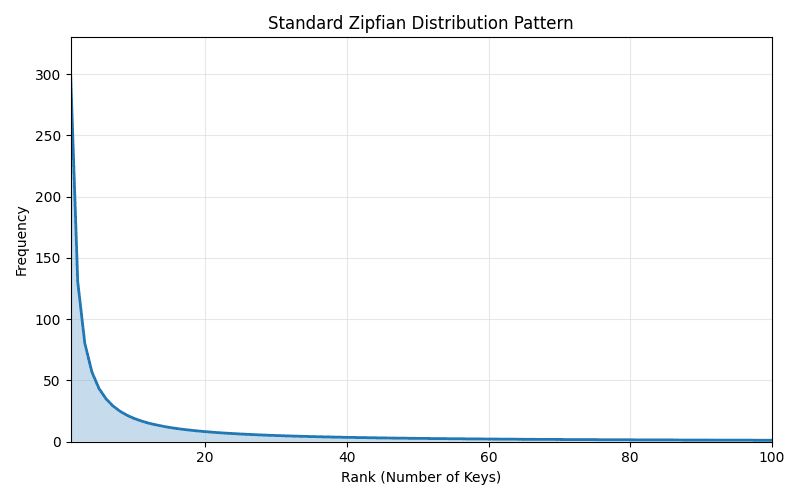
What is a zipfian distribution?

A zipfian distribution is a pattern where a small number of items appear more often that the rest of the items. It follows Zipf’s law which states that “when a set of measured values is sorted in decreasing order, the value of the n-th entry is often approximately inversely proportional to n”.

Simply, the first item will appear twice as often as the second item and three times as much as the third item. Some scenarios where this occurs is internet traffic. Popular websites visited follow a zipfian distribution. This is also observed in databases where popular tables, shards and columns get majority of the traffic.

What is rejection inversion?

Rejection inversion is a sampling algorithm for generating random variates for monotone discrete distributions.

It was first introduced in 1996 in the paper, “Rejection-inversion to generate variates from monotone discrete distributions“ by W. Hörmann and G. Derflinger, aiming to provide an algorithm that could cope with infinite tails and its generation time was not affected by the size of the domain of the distribution.

Standard rejection sampling algorithms take a hat/envelope function, suggest candidates based on the hat function and accept them if they fall within the target distribution.

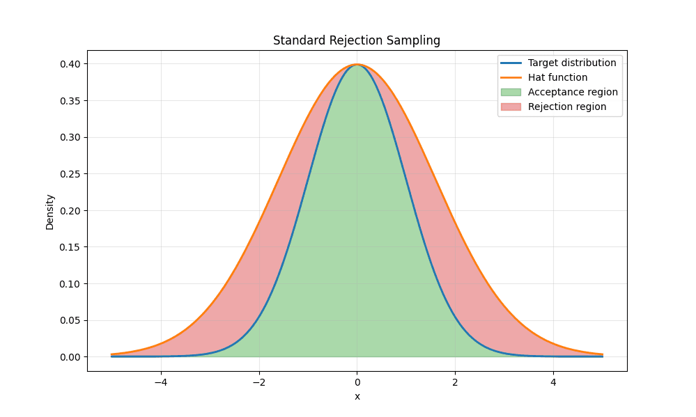
As shown above, hat function $h(x)$ will be used to suggest candidates and if they fall within the acceptance region(green) then they are accepted.

Given the simple gaussian distribution shown it is quite easy to generate values that fall in the acceptance region. However in more complex distributions like Zipfian, it will lead to a high number of rejected candidates, slowing down the algorithm.

Rejection inversion creates a continuous approximation of the cumulative distribution and combines inversion with rejection sampling to efficiently accept or reject candidates. This statement might sound daunting so let’s explore.

Let’s take a look at an example of the number of keys in a B-Tree node with an order(m) of 11. This means each node can only have a maximum of 10 keys (m-1). These are discrete values. The number of keys can only be whole numbers between 0 and 10(inclusive) so we do not expect 5.5 keys.

Assuming a zipf distribution, the histogram would look like this:

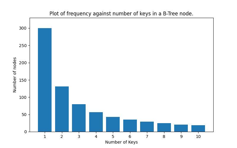
Most nodes would have a few keys(1 or 2).

A continuous hat function for rejection inversion would look like this.

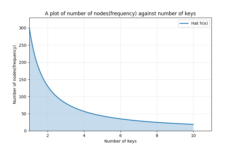
Instead of discrete values we have continuous values that we can sample from.

The hat function is used to calculate the Cumulative Distribution Function(CDF) through its integral. Generally, the hat function chosen has a well defined integral.

$$H(x) = \int_o^x f(x)\, dx$$

The CDF would look like this:

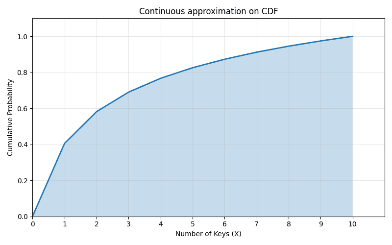
The CDF( $H(x)$ ) always adds up to one. Hence to get a discrete sample value, we generate a random uniform value $U \in [0, 1]$ between 0 and 1, and map it to a the cumulative distribution then calculate the inverse CDF ($H^{-1}$).

The inverse CDF gives us a float value $X$.

$$X = H^{-1}(x)$$

This sample is rounded to the nearest integer($k$) given we are generating discrete values, and taken through an acceptance check to reject or accept it.

$$K \leftarrow \lfloor X + \frac{1}{2} \rfloor$$

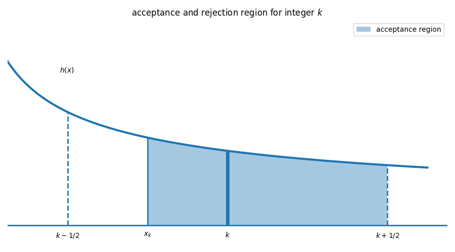
$k$ is within an integer bucket between $k - \frac{1}{2}$ and $k + \frac{1}{2}$. The checks ensure that $k$ falls within the acceptance region $(x_k \rightarrow k + \frac{1}{2})$; otherwise, it will be rejected.

The normal discrete CDF is a step function (checkout previous CDF blog) and is slow to inverse especially for long tailed distributions hence the continuous approximation serves as a better function.

The general algorithm is as follows:

1. Generate a random uniform value $U \in [0, 1]$
2. Map $U$ to an area on the continuous approximation.
3. Find $X = H^{-1}(U)$.
4. Round to nearest integer: $K \leftarrow \lfloor X + \frac{1}{2}\rfloor$.
5. Accept or reject if $k$ passes the squeeze or acceptance check.

Generating random values for zipfian distribution

For zipfian distributions, we use the probability function below:

$$P_k = (v+k)^{-q}$$

Where:

$$q > 1\quad and \quad v > 0$$

$q$ represents the zipfian exponent and determines how skewed the distribution will be while $v$ is the offset that shifts the distribution left or right - we'll observe this later.

The integral of the hat function $h(x)$, is used to create a continuous approximation of the CDF.

$$H(x) = \exp((1-q) * \ln(v+x)) * (\frac{1}{1-q})$$

While its inverse is used to get a random value X on the x axis.

$$H^{-1} = -v + \exp(\frac{1}{1-q}) * \ln((1-q) * x)$$

Algorithm

The rejection-inversion paper gives us a well defined algorithm to generate zipfian variates. $q$, $v$ and $i_{max}$ are inputs.

1. Computer and store $1-q$,$\,$ $\frac{1}{1-q}$

2. Define:

   $$H(x) = \exp((1-q) * \ln(v+x)) * (\frac{1}{1-q})$$
   $$H^{-1} = -v + \exp(\frac{1}{1-q}) * \ln((1-q) * x)$$

   as macros or functions.

3. Compute and store:

   $$H(x_o) = H(\frac{1}{2}) - \exp(\ln(v) * (-q))$$ $$s = 1 - H^{-1}(H(\frac{3}{2}) - \exp(\ln(v + 1) * (-q)))$$

4. While true:

   a. Generate uniform random number $U \in [0, 1]$

   b. Set $U = H(i_{max}+\frac{1}{2}) + U*(H(x_o) - H(i_{max} + \frac{1}{2}))$.

   This step maps the random number $U$ to an area in the cumulative distibution.

   c. Set $X = H^{-1}(U)$

   d. Round $X$ to nearest integer and set its value to $K$.

   e. $If \,(K-X \le s)$, then return $K$; This is a cheap check (squeeze) to accept the candidate if valid. If not, we proceed to f.

   f. $Else \,if\, (U \ge H(K + \frac{1}{2}) - \exp(-\ln(v + K) * q))$, return $K$; This is the full check. If candidate passes it’s accepted else the loop continues.

Choosing $q, v$ and $i_{max}$

$i_{max}$ represents the maximum discrete generated value expected in the distribution. All values generated will fall below this.

$q$ controls skew of the distribution. In simpler terms, it controls how steep the distribution is. A smaller value of $q$ generates a heavier tail.

$v$ controls how many of the values are concentrated towards the beginning, essentially shifting the distribution left or right along the x-axis.

The diagram below shows different choices of $q$ and $v$ with $i_{max} = 50,000$ and how the distribution turns out.

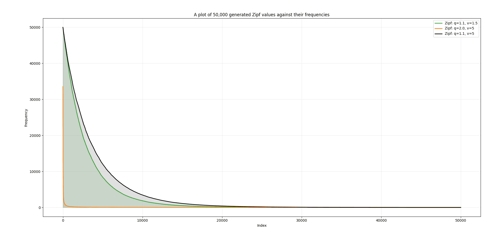
Comparing $v = 1.5$ (green) and $v = 5$ (black), we can see that a higher value of $v$ shifts the graph to the right, giving more values a higher frequency.

As for $q$, comparing $q=1.1$ (green) and $q = 2.0$ (orange) we see that a smaller $q$ produces a heavy tail where the probability of larger values is higher and $q=2$ produces a subquadratic tail.

Altering values of $q$ and $v$ will generate your desired pattern.

What advantages does rejection inversion offer?

1. Rejection inversion requires half the uniform random numbers compared to standard rejection
2. Rejection inversion can be used to sample from distributions with classical tails as well as heavy tails.
3. The additional squeeze helps avoid expensive calculations while performing acceptance checks.

Conclusion

Rejection inversion helps us sample from discrete monotone distributions while providing great performance compared to other sampling algorithms.$It is widely used in benchmarking storage engines as well as standard libraries like Go's math library. Now that we understand the theory behind it, we'll take a look on how we can use it in the next blog.

Thanks for reading. Got any enquiries, corrections or comments? Feel free to reach me at [email protected] or on LinkedIn.

Resources

Here are some resources I think you might find useful to understand this further:

1. Rejection-inversion paper by W. Hörmann and G. Derflinger.
2. Rejection Sampling video.
3. Inverse Transform sampling video.