Cumulative Distribution Function (CDF)

What is CDF?

A Cumulative Distribution Function describes the probability that a random variable $X$ is less than or equal to a specific value $x$ .

F_X(x) = P(X <= x)

It is the cumulative probabilities of all items up to $x$ . It is universal for both discrete and continuous values. For discrete distributions, to get the CDF you would sum up all probabilities of items $\le x$ .

\sum_{X \le x} P(X = x)

For continuous distributions, CDF is calculated by getting the integral of the curve upto point $x$ .

P(x) = \int_{- \infty}^x f(x)\,dx

This is also the area under a PDF curve with $x$ and $- \infty$ serving as the boundaries.

Given that the CDF is a sum of probabilities, it always maxes out at 1.

Let’s look at two examples:

Suppose we have a dice. Every time we roll a dice we expect to get a value 1 - 6. The probability of getting each number is $\frac{1}{6}$ .

Suppose we want to know the probability of rolling 1, 2 and 3?

P(X \le x) = \frac{1}{6} + \frac{1}{6} + \frac{1}{6} = \frac{1}{2}

We have summed up the probabilities of 1, 2 and 3. The diagram below plots this CDF:

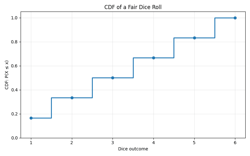
We start at probability of rolling 1 being $\frac{1}{6}$ , and as we progress, we add up the probabilities of rolling all the other numbers.

At 5, the CDF will be the probability of rolling 1, 2, 3, 4 and 5, which is the sum of all other probabilities prior.

P(X \le 5) = \frac{1}{6} + \frac{1}{6} + \frac{1}{6} + \frac{1}{6} + \frac{1}{6} = \frac{5}{6}

Let’s now look at a continuous distribution.

Suppose we have probabilities of different times that the sun will rise in different seasons year round. Depending on when and where you are in the world, this may be any time between 4am and 9am. The diagram below represents it's PDF(Not familiar with PDF? check it out here).

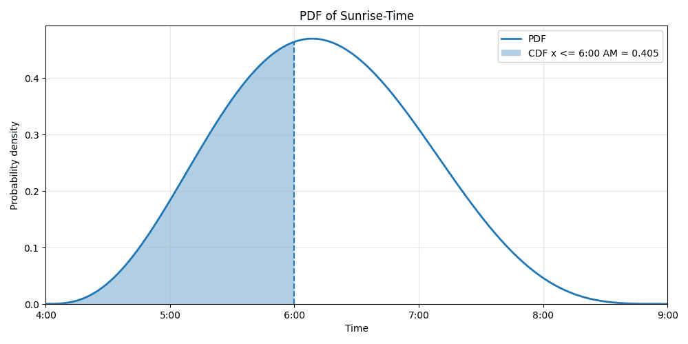
The probability that the sun rises before 6am is indicated by the shaded area. This is the CDF.

P(X \le 6) = \int_{-\infty}^6 f(6)\, dx

The CDF graph would look as shown below

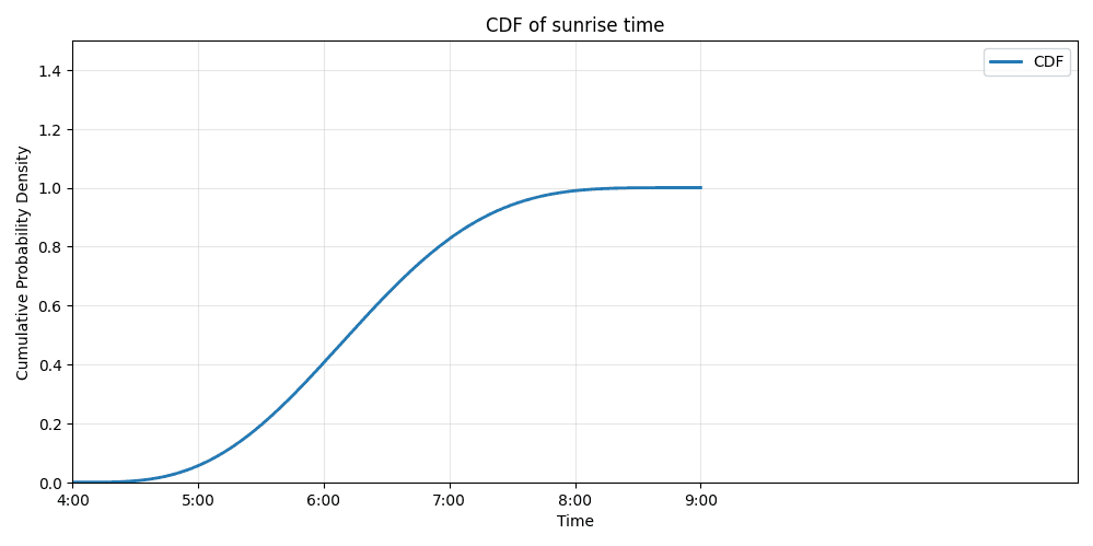
The CDF looks different for different distributions but the common thing is that they flatten out at $1$ as that is the maximum expected sum of all probabilities

Inverse CDF

The inverse CDF ( $P^{-1}$ ), also known as the quantile, is used to get the random value associated with a particular CDF value.

Take a look at the graph above(CDF of sunrise time), if you select a random CDF value on the y-axis, the inverse CDF will give you a value on the x axis. Values yielded follow the distribution on the CDF.

It is commonly used in different sampling techniques like inverse transform and rejection inversion, to get random numbers from a given CDF.

Continuous distributions are simpler to inverse than discrete given that they have a smooth curve hence sampling techniques like rejection inversion create a continuous approximation to make sampling easier.

In sampling literature, you will frequently encounter inverse CDF being part of generators that produce values matching certain distributions. This is necessary when generating workloads in testing and benchmarking of software systems to model different real world patterns.

Thanks for reading. Got any enquiries, corrections or comments? Feel free to reach me at [email protected] or on LinkedIn.