PMF and PDF explained

Introduction

Probability Mass Function and Probability Density Function are two terms commonly used in probability and statistics as well as overlaping areas in Computer Science. What do they mean and how can we visualize them? Let's take a look.

What is Probability Mass Function?

A probabiliy mass function is a function that gives the exact probability of a random discrete variable $X$ being equal to a value $x$ .

A probability mass function is exclusively for discrete random variables. It is written as:

$P(X = x) = 0.3$

This is read as “the probability that a random discrete variable $X$ is equal to $x$ is 0.3”.

Let’s look at an example:

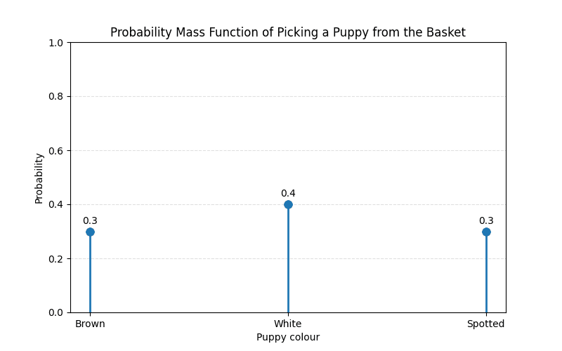
Suppose we have a litter of 10 puppies - three brown, four white and three spotted. We then place them in a basket, close our eyes and pick one at random.

We have three possible scenarios for each pick. We either pick a brown, white or spotted puppy. Lets issue them ids 1, 2 and 3 respectively. These act as our discrete values. We do not expect to pick a puppy that’s both white and brown.

$x = { 1, 2, 3 }$

The probability of each puppy being picked:

Brown (1) - 0.3
White (2) - 0.4
Spotted (3) - 0.3

The probability that a random pick will result in picking a brown puppy will be written as:

$P(X=1) = 0.3$

The PMF graph would look like this: pmf_illustration

What is Probability Density Function (PDF)?

We have seen that PMF deals with discrete random values. Probability Density Function deals with continuous random variables. It gives the probability that a random value $X$ is within a certain interval.

Take an example with a plot of probability density of people’s height in centimeters.

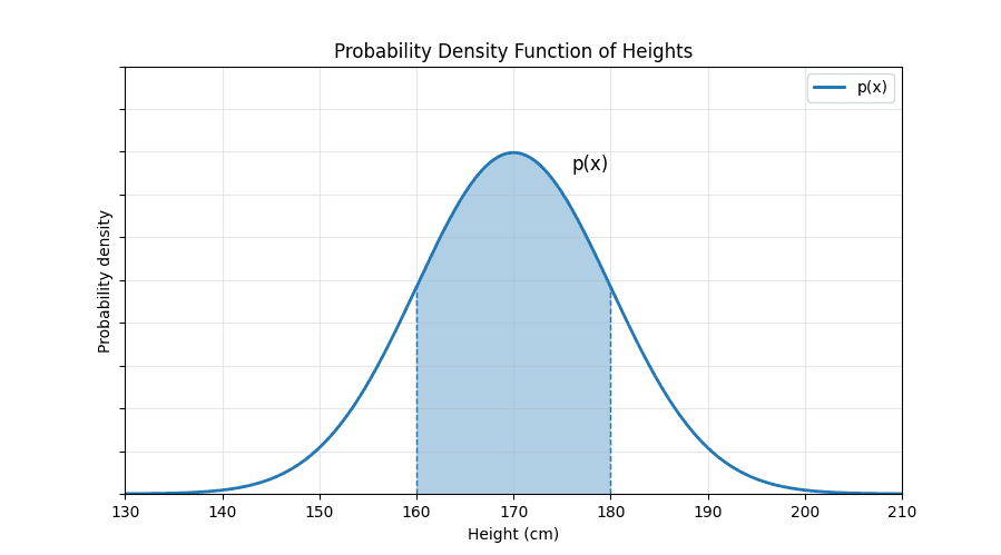
The value of height is continuous, could be 170cm or 170.5cm.

The probability that a random person’s height is between 160 cm and 170cm is the area under the curve between the intervals.

p(a \le x \le b) = \int_a^b p(x)\,dx

Where:

a = 160, b = 170

Given that we are dealing with continuous values, the probability of a specific point is always zero since probability of continuous values is always evaluated over a range, and the width of a single point is zero.

P(X = x) = 0

PMF and PDF for common distributions are usually well defined. For example the PDF of a exponential distribution is:

f(x) = \lambda e^{-\lambda x}

And the unnormalized PMF for a zipfian distribution is:

p_k = (v + k)^{-q}

Where

k = 0, 1, 2

q \gt 1, v \gt 0

Conclusion

Probability Mass Function(PMF) and Probability Density Function(PDF) are two concepts used to describe probability distributions and come in handy in different areas of Computer Science.

Thanks for reading. Hope you learnt a thing or two. Got any enquiries, corrections or comments? Feel free to reach me at [email protected] or on LinkedIn.