Why B+ Trees Still Matter in the Age of Cloud Databases

Introduction

Over the past 15 years, we have seen a rise in distributed cloud databases offered by various providers - Amazon’s DynamoDB, Aurora, RDS, Azure CosmosDB, supabase etc - arguably kickstarted by Amazon’s Dynamo paper in 2007 which showcases the design and implementation of a highly available key-value store to handle the extreme scale of their ecommerce store.

Cloud databases promise of scalability without worry, while attractive, does not absolve us of the responsibility of choosing efficient index structures. Under the hood, cloud databases rely on the same storage structures and an understanding of how they work will help you make better design choices that improve performance, reduce costs and increase customer satisfaction.

Categorization

There are two categories of cloud databases:

Managed databases which use open source solutions like PostgreSQL and handle replication, backup, snapshotting, access control and scaling your database based on demand.
Proprietary Databases that have been developed by cloud providers, or sometimes have taken open source solutions and modified them for a specific purpose. Good examples are Azure Cosmos DB and Amazon Aurora.

Both of these category of databases tend to utilize the same structures that have been battle tested and innovate around them. These are B-Trees and Log-Structured Merge Tree (LSM Trees).

The main difference in choosing either is that B-Trees are optimized for read-heavy workloads due to their balanced, sorted and disk-efficient structure while LSM Trees are optimized for write-heavy workloads since they require appending to a commit log and writing into an in-memory structure - memtable.

In this edition, we will explore B+ Trees, a variation of B Trees, and how understanding how they work can help you make better technical and business decisions.

Core Database Performance: Index Structures

Role of Indexes

James is a computer science major at MIT and he needs to find a specific computer science book. He visits the library but does not know the exact section or shelf the book is located.

James has two options:

Walk through every shelf in the library checking every book until he finds the book. This could take hours or days, given the size of the library.
Check the catalog and locate the exact position of the book, then walk straight to the shelf and retrieve the book. This will probably take a few minutes.

Effectively, the catalog has helped James know the location of the book without having to go through all the shelves.

In databases, the catalog is equivalent of an index. An index stores information on where specific data is stored on disk. Indexes have a unique key which is used to identify the resource, in James’ case it would be the book title, and choosing the right key will also influence how efficient retrieval will be (we explore this later in the blog).

For efficient retrieval (lookup) where you have billions of records, you need efficient structures, both in-memory and on disk. B-Trees have been the preferred choice among majority of database engines and continue to prove as the best choice for such situations. Let’s explore what exactly are B-Trees and what role they play in indexing.

What are B-Trees?

In computer science, Trees are a way or organizing data in a hierarchical structure that looks like a family tree or a root system.

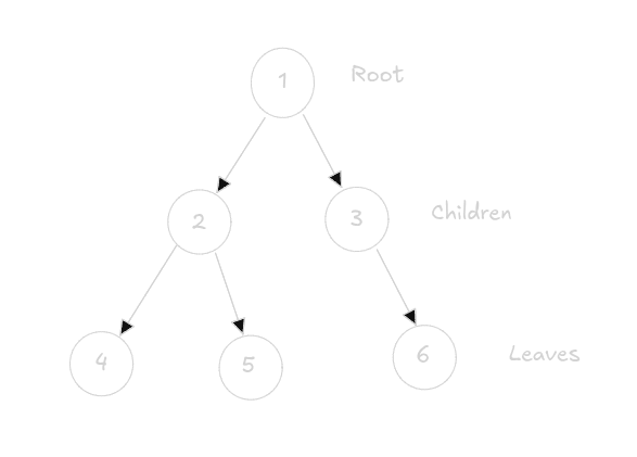
The top-most node is called the Root Node and each node can have n number of nodes arranged in a specific way. Special kinds of trees exist (binary trees, B-trees, AVL trees, etc.), each with rules about how nodes are arranged.

Binary Trees only have nodes constrained to two children.

To locate a node, one has to start from the root node and traverse through the tree until the node is located. In order to make this process efficient, Binary Search Trees add a constraint that values on the left child must be less than the parent’s value and values on the right child must be greater than the parent’s value. This means that looking for a value cut’s the items to check by half on each step, and provides a time complexity of O(logn).

The downside of Binary Trees is that tree height increases as nodes are added. This translates to additional comparisons and impacts performance. But what if we could have more than two child nodes?

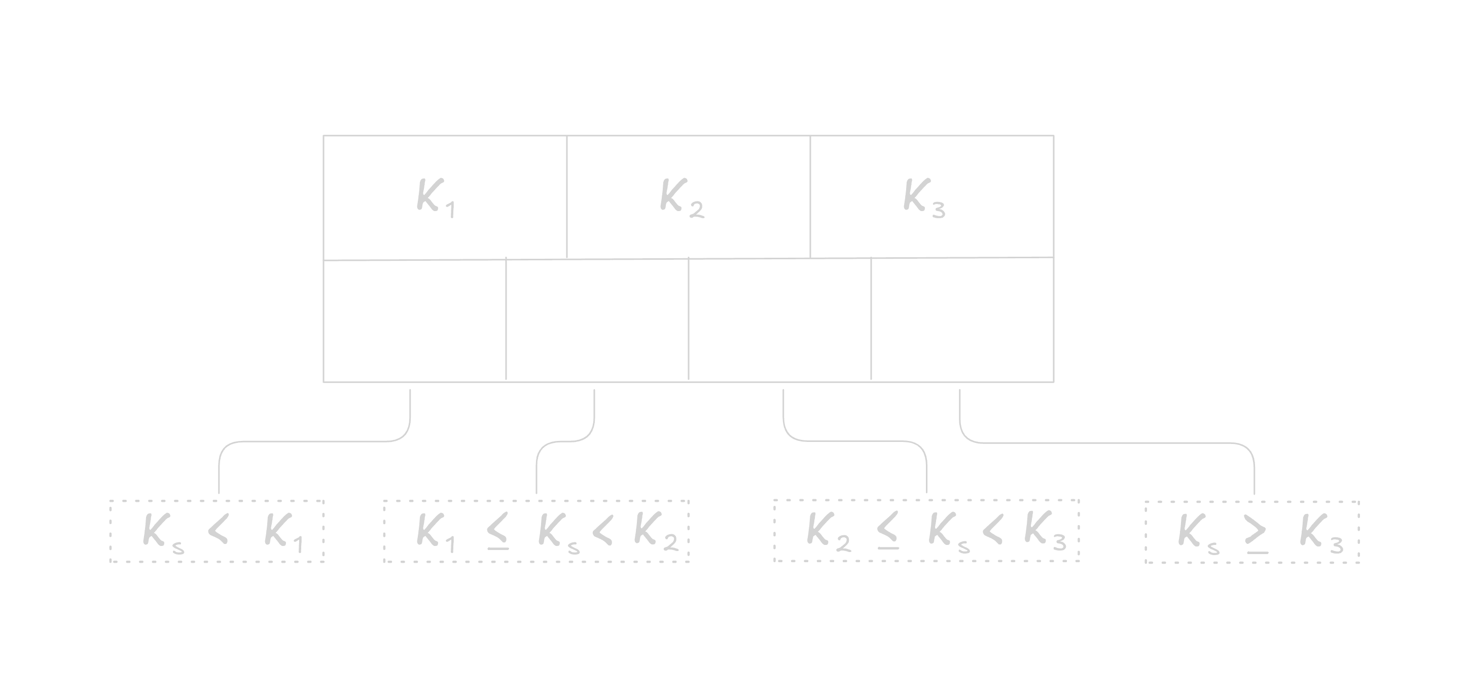
Introducing B-Trees. In B-Trees nodes can have more than two children (referred to as fanout). A B-Tree structure contains n Keys(also known as separator keys) and n+1 Pointers to child nodes.

Each of the pointer references a child node with the same structure.

Keys in a B-Tree are kept in a sorted order. This ensures that lookup algorithms with good time complexity like binary search can be used to retrieve the key.

The variable number of keys also help in reducing the height of the tree, reducing the number of steps needed to retrieve a value.

B-Tree nodes can either be Internal nodes or Leaf nodes. Internal nodes store keys and pointers to child nodes - functioning as a guide to leaf nodes - while leaf nodes store keys and values and have no children.

What are B+ Trees?

B+ Trees are a variation of B Trees that only store values on the leaf nodes, whereas B-Trees can also store values on internal nodes. Essentially internal nodes only serve as guides to the leaf nodes. Due to this, all operations (inserting, updating, removing and retrieving data records) only affect leaf nodes and propagate to higher levels only during splits and merges.

B+ Trees leaf nodes are also linked in a linked-list manner, making range queries much faster.

Constraints

On various literature, internal nodes can have upto n Keys, which is referred to as the order of the node and a minimum of k keys, referred to as the degree. The root node can have between 1 and 2k(or n) keys.

When the number of keys goes above the order of the node, it has to be split. Conversely, when the number of keys goes below k, the node has to be merged with the adjacent node to ensure constraints are met.

Pointers to child nodes are arranged in accordance with their corresponding keys. The first pointer in the node points to the child node holding items less than the first key, and the last pointer in the node points to the subtree holding items greater than or equal to the last key. Other pointers reference subtrees between the two keys as shown below.

In another variation of the B+ Tree called B-link Tree, a high key is introduced to act as the upper boundary for the node, ensuring that there are n keys and pointers in internal nodes, making storage and retrieval on-disk much more efficient.

Splits and Merges

Splits and Merges maintain the constraints and keep the B+ Tree balanced at all times.

Suppose we want to insert 31 in the following B+ Tree with an order (n) of 3:

31 is greater than 25, this will direct us to the child node referenced by p2. However, this node is already full (order of 3). The node will have to be split.

Splits are done by allocating the new node, transferring half the elements from the splitting node to it, and adding its first key and pointer to the parent node. They key will be promoted. The index at which the split is performed is called the split point or midpoint.

Our new tree now looks like this:

They key 30 is now promoted to the parent node. If the parent node was also full it would also have to be split. If all internal nodes in the traversal path we full, this process would propagate upwards to the root node and the root node would have to be split as well, and a new root node would be allocated.

For internal nodes, splits involve creating a new node and moving elements from index n/2 + 1 to it. The split point key is promoted to the parent. The image below demonstrates the split process during inserting the new element 26

Internal node splits usually propagate from the leaf nodes.

Merges are as a result of deletions that leave too few keys on a node. This is called an underflow. There are two scenarios for underflows.

Two adjacent nodes have a common parent and the total number of keys between them can fit in one node. Their contents should be concatenated.
Two adjacent nodes have a common parent but their keys do not fit on a single node. Their contents should be redistributed between the nodes. This is called Rebalancing.

Nodes are merged if they satisfy the following conditions:

For leaf nodes: If a node can hold n key-value pairs and the total count of key-value pairs on neighbouring nodes is less than or equal to n.
For internal nodes: If a node can hold n+1 pointers and the total count of pointers on neighbouring nodes is less than or equal to n+1

For leaf nodes, merging involves concatenating items from the right node to the left. The number of pointers on the parent node will reduce since the right child will be deleted. On internal nodes, the separator key will have to be moved from the parent to the left node - demoted, and If the parent is left with less children it will also have to be merged. This process can also propagate to the root and may end up in reducing the tree height. Below shows merging after deletion of key 16:

Below is a demonstration of merging internal nodes as a result of deleting key 10.

On disk structure

Now that we understand the basic semantics of how B-Trees work, let’s see how they’re represented on-disk. When working with on disk data structures, access is a bit different from in memory data structures. We have to come up with efficient binary file formats that fit with the physical layout of storage devices since locality, especially in databases, reduces the seek time. An inefficient file format will increase the time it takes to read and write data, due to increased seek time, which will eventually cascade to client’s response time.

Database systems store data in data and index files partitioned in fixed-size units called pages. Pages have sizes that range from 4 to 16 Kb - PostgreSQL uses 8Kb pages while MySQL has 16Kb pages. Each B-Tree node is stored on it’s own page. Pages are subdivided into slots that store information on the node and can be arranged in such a way that allows storage of variable size data. These specific structure is called a slotted-page.

A slotted-page contains a fixed-size header that holds the node’s metadata - LSN, checksums, CRC etc., data cells that hold the actual data and cell pointers that hold the offset to the actual data cell they represent. The diagram below shows the layout of a slotted-page:

Cell pointers are inserted from lower offsets (beginning of the page) while cells are inserted from the higher offsets (end of the page). Cells pointers are used to maintain lexicographical order of the cells and are used to perform binary searches when retrieving cells. In case cell offset changes, like during a rewrite, garbage collection or defragmentation, the new offset can be updated on the cell pointers.

The free space between pointers and cells is meant to accommodate additional, variable-size cells, given that we do not know beforehand what size cell will be added. The amount of free space available and the offset of the free space is stored in the page header. This makes it faster to access and update.

Here is PostgreSQL’s page layout. Similar to our previous diagram:

In case a new cell needs to be added but there isn’t enough space:

If the cells are fragmented - contain empty spaces in between - and the total empty space can accommodate the new cell, the node is defragmented - cells are rewritten to contiguous locations to eliminate any empty spaces in between cells. After this process, the new cell is now inserted.
If the total free space cannot accommodate the new cell, an extra page, same size as the primary page, is created. This page is called the overflow page. The extra cell can be inserted in the overflow page. SQLite describes how they implement this here

Cell Layout

Within a cell, we have a distinction between cells that hold keys and cells that hold values. Ideally, we need to have the following items to compose a cell:

Key Size
Value Size in the case of leaf nodes
Cell type
Key bytes
Value Bytes
ID of child page for internal nodes. This can be the offset of the child page or store the page ID in lookup table that you use to map to a specific address.

The images below show possible layouts for variable-size cells that hold data records and ones that do not(internal nodes).

Visualization

Now that we understand the inner workings of B-Trees both in-memory and on disk, we can look at an example at how this looks on an actual database. For this exercise, we will use PostgreSQL.

PostgreSQL stores data in the cluster’s data directory, commonly referred to as PGDATA. Common locations include /var/lib/pgsql/data or /var/lib/postgresql/<version>/main/base.

If you ls into the storage directory you will find numbered directories, representing databases created.

ubuntu@ubuntu:~$ ls /var/lib/postgresql/16/main/base
1  4  5
ubuntu@ubuntu:~$

Each of the directories contain comprise of index files and data files(known as heap files in Postgres). Each table in a database has it’s own heap file and index file. The index files use a B-Tree structure to store and retrieve data from heap files while heap files are simply used for storing data and metadata.

ubuntu@ubuntu:~$ ls /var/lib/postgresql/16/main/base/4
112	      13478_fsm  13493_fsm	2600	    2605_vm     2610_vm   pg_filenode.map
113	      13478_vm   13493_vm	  2600_fsm  2606	      2611      PG_VERSION
1247	    13481      13496	    2600_vm   2606_fsm    2612
1247_fsm  13482      13497	    2601	    2606_vm     2612_fsm
1247_vm   13483      1417	      2601_fsm  2607	      2612_vm
1249	    13483_fsm  1418	      2601_vm   2607_fsm    2613
1249_fsm  13483_vm   174	      2602	    2607_vm     2615
1249_vm   13486      175	      2602_fsm  2608	      2615_fsm
1255	    13487      2187	      2602_vm   2608_fsm    2615_vm
1255_fsm  13488      2224	      2603	    2608_vm     2616
1255_vm   13488_fsm  2228	      2603_fsm  2609	      2616_fsm
1259	  1 3488_vm    2328	      2603_vm   2609_fsm    2616_vm
1259_fsm  13491      2336	      2604	    2609_vm     2617
1259_vm   13492      2337	      2605	    2610	      2617_fsm
13478	    13493      2579	      2605_fsm  2610_fsm    2617_vm
ubuntu@ubuntu:~$

Since these files are in binary format, we will use pg_filedump to read and interpret their contents.

First let’s install pg_filedump:

On linux

sudo apt update 
sudo apt-get install postgresql-filedump

On Windows and MacOS

Clone the repo and follow the installation instructions:

git clone https://git.postgresql.org/git/pg_filedump.git

Now, navigate to your postgresql data file and read the contents of one of the file.

sudo pg_filedump -i  /var/lib/postgresql/16/main/base/4/2604 | head -n 50

This is the output we get:


## ******************************************************************\
## * PostgreSQL File/Block Formatted Dump Utility
## \
## * File: /var/lib/postgresql/16/main/base/4/2604
## * Options used: -i
## ******************************************************************\

## Block    0 *******************************************************\
## \<Header\> -----
## Block Offset: 0x00000000         Offsets: Lower      72 (0x0048)
## Block: Size 8192  Version    4            Upper    8176 (0x1ff0)
## LSN:  logid      0 recoff 0x010053b8      Special  8176 (0x1ff0)
## Items:   12                      Free Space: 8104
## Checksum: 0x0000  Prune XID: 0x00000000  Flags: 0x0000 ()
## Length (including item array): 72

## BTree Meta Data:  Magic (0x00053162)   Version (4)
## Root:     Block (1)  Level (0)
## FastRoot: Block (1)  Level (0)

## \<Special Section\> -----
## BTree Index Section:
## Flags: 0x0008 (META)
## Blocks: Previous (0)  Next (0)  Level (0)  CycleId (0)

## Block    1 *******************************************************\
## \<Header\> -----
## Block Offset: 0x00002000         Offsets: Lower     536 (0x0218)
## Block: Size 8192  Version    4            Upper    3824 (0x0ef0)
## LSN:  logid      0 recoff 0x01005328      Special  8176 (0x1ff0)
## Items:  128                      Free Space: 3288
## Checksum: 0x0000  Prune XID: 0x00000000  Flags: 0x0000 ()
## Length (including item array): 536

## \<Data\> -----
## Item   1 -- Length:   32  Offset: 8144 (0x1fd0)  Flags: NORMAL
## Block Id: 0  linp Index: 32  Size: 32
## Has Nulls: 0  Has Varwidths: 1

## Item   2 -- Length:   24  Offset: 8120 (0x1fb8)  Flags: NORMAL
## Block Id: 0  linp Index: 34  Size: 24
## Has Nulls: 0  Has Varwidths: 1

## Item   3 -- Length:   32  Offset: 8088 (0x1f98)  Flags: NORMAL
## Block Id: 0  linp Index: 49  Size: 32
## Has Nulls: 0  Has Varwidths: 1

This is an index file. We can see the <Header> section just at the beginning of the block. This header stores:

Block offsets - The offset of the page.
Block Size
Log Sequence Number (LSN)
Number of items(cells) stored.
Free space offsets - Upper and lower offsets of the free space.
A checksum or Cyclic Redundancy Checks(CRC) used to check integrity of the data.
Extra metadata like a magic number.

On Block 1, we can see data output as well:

## \<Data\> -----
## Item   1 -- Length:   32  Offset: 8144 (0x1fd0)  Flags: NORMAL
## Block Id: 0  linp Index: 32  Size: 32
## Has Nulls: 0  Has Varwidths: 1

This represents a cell. We can see it stores the block ID, size of the data, offset of the data, some flags (you can set flags with bitmasks and bitwise operations) among other extra metadata.

If you would like to access the raw hex content of the file you can run pg_filedump with the -f flag:

sudo pg_filedump -i -f /var/lib/postgresql/16/main/base/4/2604 | head -n 50

Back to Indexes

Now, how exactly does indexing affect performance?

First, we need to understand right-only appends. When you create a table, you have to select a column as a primary key. In a lot of cases, the primary key chosen increases monotonically (Autoincrement). This means that when inserting into the B-Tree, all new values will be inserted on the right most node since every new key will be the largest key. This also means non-leaf pages are less fragmented and splits or rebalances do not occur as often.

You can also optimize this by caching the right-most leaf node. On new entries, if the cached node has enough free space to accommodate a new entry and the insertion key is strictly greater than the first key in this page, you can simply search within the cached block and insert the key at the appropriate location skipping the whole read path. PostgreSQL calls this fastpath and SQLite’s similar concept is quickbalance.

If the chosen indexing key is random, like UUID v4, this optimization is not possible and results in random inserts and possibly more fragmentation. Also, when splits occur, the new nodes have half as much as the order and will fill up much faster compared to SQLite’s quickbalance which allocates a new empty node less likely to fill up faster.

The second thing is size. Autoincremented primary keys occupy between 4 and 32 bits(1 - 4 bytes) depending on how many insertions have happened. UUIDs on the other hand are 128bit (16 bytes) numbers. Given the cell size and how many cells(tuples) are expected on a page - a few hundreds - this greatly reduces the number of cells that can be stored. This will result in more overflows, warranting extra overflow-pages and increasing space usage.

The two concepts also apply when choosing secondary indexes. When you create a secondary index, a new index file/B-Tree is created referencing the primary index or actual data address. If the chosen index key is large or non-sequential, you might lose out on performance or worse case, slow down queries AND consume more space.

Business Implications

Whether you are using a cloud database or self hosted, we have seen that improper indexing will lead to slower lookups and more space consumption. If you are using a cloud database, this will translate to more costs on storage and compute in an effort to speed up queries but without proper understanding of how the underlying systems work, it will not solve the root of the problem.

Slower queries lead to slower applications and increased customer dissatisfaction.

On the flip side, once you have that figured out B-Trees offer great performance for reads and range queries (remember the linked children). If you are running a Fintech platform, concurrent operations like checking account balances, fraud checks and card verifications will run much quicker.

Fast range queries provide better performance for audits and compliance checks, which involve retrieving a large, sequential datasets.

In summary, why should you care about B+ Trees and indexing?:

Lower latency
Better customer satisfaction
Faster compliance reporting
Lower compute and storage costs

Beyond B-Trees: Tradeoffs

B-Trees are excellent for read-heavy workloads and used quite often in Transactional Databases (OLTP). When it comes to write heavy workloads LSM-Trees tend to out-perform B-Trees and are better suited for Analytical Databases (OLAP) and datalakes, though do not perform as well with reads. Generally, databases come up with strategies to mitigate the downside of either, like caching strategies to speedup writes or batching writes.

Some databases combine the best of both worlds and use both B-Trees and LSM Trees and balance the strength of both structures. Some examples are CockroachDB and YugabyteDB.

Conclusion

B-Trees: hidden to users, dictate scalability. Whether in the cloud or on-prem, understanding how they work will help you optimize indexes and build performant and scalable systems.

Cloud won’t save you from bad design…so let us help :)

We engineer high performance systems that satisfy your client needs. Talk to us at devcanary.com or shoot us an email at [email protected].

References

Database Internals by Alex Petrov
Designing Data-Intensive Applications by Martin Kleppmann
B+ Tree Visualization
Amazon Aurora supported Index types blog